Digital Signal Processing
Digital Signal Processing (DSP) is primarily concerned with the representation of real-life signals in digital (numerical) form and in the interpretation, analysis and information extraction from these signals by means of computer or specialized hardware. DSP encompasses several disciplines across science and is thus very interdisciplinary and has revolutionized many different areas of science and engineering (from telephone to military, from medical to space exploration etc…). Some of its most useful and interesting applications are: image/sound filtering, speech generation and recognition, radar/sonar, seismology, computed tomography. This brief page intends to present the various algorithms available in IPredict’s library and not to explain in detail how the algorithms work or the effects of applying the algorithm to signals.
Please refer to “Signal and Systems” by Alan V. Oppenheim for a detailed explanation of the techniques implemented and of all the necessary math behind.
Wavelet and Haar Transform
The first Wavelet Transform has been invented by Alfred Haar, a Hungarian mathematician. His simple approach was to transform a signal by remembering the differences between pairs of elements forming a scale and applying the same approach recursively on each scale up to a final sum. Daubechies Wavelets are the most common discrete Wavelet Transform. They have been invented by Ingrid Daubechies, a Belgian mathematician. The approach is more complex than the Haar Transform that is indeed the Daubechies Wavelet Transform of the first order. The algorithm is basically the cascading application of quadrature mirrored filters to the input signal creating what is known as Filter Bank where each step of the filter computes a set of coefficients for each level of the Filter Bank. These coefficients constitute the Wavelet Transform.
Fourier Sine Transform and Fourier Cosine Transform
The Discrete Sine and Cosine Transforms are both Discrete Fourier Transforms that express the original signal as sum of cosine or sine functions at different frequencies. Both are transforms that use only real numbers and are essentially equivalent to their “father” the Discrete Fourier Transform.
Fast Fourier Transform
This is the well known algorithm to compute in a fast way the Discrete Fourier Transform that is used in several applications. The Fourier Transform X(k) of the time-series x(k)
is the following expression:
The Fast Fourier Transform is the algorithm that revolutionized the field of Digital Signal Processing because of its “fast” nature. The algorithm indicated above is while the fast version is only that is much faster. See this page on Fast Fourier Transform for further information.
Fourier Power Spectrum
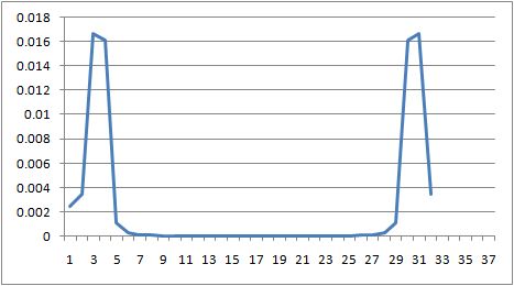
The Fourier Power Spectrum or Power Spectral Density of a signal is a real function that expresses the energy of the signal per single component frequency. This is normally called the spectrum of a signal. Its computation is simple and is the product of the Fourier Transform of the signal and its complex conjugate. In symbols:
where represents the complex conjugate of the signal. An example power spectrum of a simple sinusoidal wave is the following:
Complex Discrete Fourier Transform
This is the general Discrete Fourier Transforms that can take as parameter complex valued signals and returns complex valued transforms. The algorithm is computed using the original algorithm and thus is “slow” compared to its “fast” couterpart but can compute arbitrary length transforms and use also complex numbers as input.
Hilbert Transform
The Hilbert Transform has been invented by David Hilbert and is a basic tool used to derive the analytic representation of the signal. It is basically computed as the convolution between the signal itself and the function .
Analytic Signal
The analytic representation of a signal is normally used in Digital Signal Processing since it gives access more easily to many properties of the signal itself. The Analytic Signal can be used to compute the Instantaneous Frequency of a signal and to apply modulation and demodulation (signal envelope) techniques. The basic idea of the analytic representation for real valued functions is that we can entirely ignore the negative frequencies of the signal.
The inverse Fourier transform of the function:
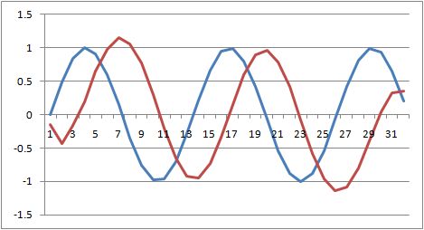
where X(f) is the Fourier transform of x(t), our signal, is then the Analytic Signal. The Analytic Signal can also be expressed as:
where A(t) is normally called Aplitude Envelope and is the instantaneous phase of the signal. The first derivative with respect to time of is the Instantaneous Frequency. You can see an example Analytic Signal of a simple sinusoidal signal of frequency 0.5:
from which the Instantaneous Frequency can be derived:
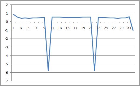
It is easily seen from this last image that the original signal had a frequency of 0.5.
Spectral Windows
Spectral windows are used to filter the signal specifically for the Spectrogram and Short Time Fourier Transform. In our library we implemented the following Spectral Windows (N is the window width):
Rectangular
Hamming
Hanning
Kaiser
Where I is the zero-th order modified Bessel function of the first kind and is a parameter whose default value is
Nuttall
Blackman
Harris
Bartlett
Barthann
This is a modified Bartlett-Hann window
Papoulis
Gauss
Where K is a parameter that varies the shape of the gaussian whose default value is 0.005.
Parzen
Is the window defined by the Parzen polynomial equation.
Hanna
Where L is a parameter that controls the shape of the window whose default is 1.0.
Spline
Is the window defined using a polynomial sine wave function similar to the Hanna window. This window function uses two parameters to control the shape of the window, the first parameter is a multiplier of the frequency of the sine wave and the second the power of the sine wave polynomial.
Short-Time Fourier Transform
The Short-time Fourier transform is a time-frequency distribution that is computed as a sliding Fourier transform on a windowed signal computed multiplying the chosen spectral window by the signal itself. The Short-time Fourier transform shows how the various spectral components of a signal vary over time.
The discrete-time Short-time Fourier transform is computed using the following formula:
where x(k) is the original signal and w(k) is the spectral window function used. You can think of the short-time Fourier transform as a moving discrete Fourier transform. Its purpose is to identify frequency changes in the underlying signal when the signal is non-stationary (when the signal is stationary a simple Discrete Fourier transform is enough to describe the spectral contents of the signal).
Spectrogram
The Spectrogram is one common way in which the Short-time Fourier transform is used. It represents the spectral densities of the signal under investigation. Its formula is the following:
where STFT is of course the Short-time Fourier transform of the original signal. This is how a spectrogram of a chirp signal appears:
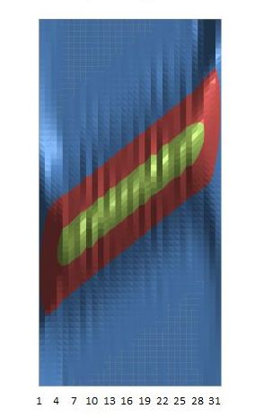
(this chirp signal has been designed so that the frequency rises linearly with time as can be clearly seen from the spectral representation).
Wigner-Ville Time-frequency Distribution
The Wigner-Ville time-frequency distribution is functionally equivalent to the Spectrogram. We chose to use the analytic signal instead of the real signal as input to the transform to reduce the artifacts generated by the transform. The basic formula used is the following:
where X(t) is the analytic companion of the real signal x(t) and is its complex conjugate.