Moving Averages

The moving averages (MA) algorithms are the classical forecasting algorithms that have been used for decades in the forecasting field. They are basically simple algorithms that can even be computed by hand (and this is why they have been so popular in the past when computers were not available to the general public).

All the Moving Averages algorithms share some common trait:

• They smooth the curve.
• They introduce some lag in the calculation so that the MA lags the original signal.
• They cut the highest frequencies (i.e. numerically they are low pass filters).

Several variations exist of the same basic algorithm that essentially computes a weighted sum. Each past term is multiplied by a constant or variable quantity and the result summed up to give the MA value:

where the term $W_t$ represents the weight of the single historical sample $X_t$

The Simple Moving Average is an equally weighted sum of the previous k historical sample where each weight $W_t$ equals $1 \over k$ for each historical sample, you can think of it as multiplying the signal by a rectangular “window” whose height is $1 \over k$ that moves as the moving average moves.

Where k is the smoothing window or period.

The Triangular Moving Average is an average that is weighted with weights that rise from the most recent sample towards the farthest sample. So in effect the weighting function is a triangle that moves as the moving average moves. The triangle is wide k units and its height is $2 \over k$ units so that the area of this triangle is 1. This gives the last historical values a higher weight and to old values a lower weight.

The Exponential Moving Average is a weighted average whose weights are exponentially decreasing from more recent historical samples to older historical values.

where $\alpha$ is the smoothing factor. To compute an $\alpha$ factor that is roughly equivalent to the simple moving average window we can use the simple formula:

where k is the window length.

Lag Factor in Moving Averages

As stated above every MA introduces a lag in the computed curve. This lag can be very annoying and depending from the application we’re dealing with can render the whole average unusable. Unfortunately there is no possible computation that drastically reduces this lag, we can only take some simplified path or use some “trick” that can reduce the lag at the expense of other approximations introduced in the computation. Most MA algorithms introduce a lag that roughly equals half of the length of the computational window i.e. $k \over 2$.

Below you can see an example of the lag introduced by a simple moving average:

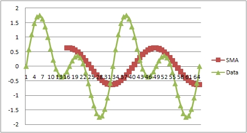
As you can see the SMA peaks are shifted to the right with respect to the peaks in the data.

Moving Averages Are Digital Low-pass Filters

A low-pass filter is a computation or a device that allows frequencies lower than the cutoff frequency to pass through the filter and reduces the frequencies higher than the cutoff frequency. We can understand why MA are low-pass filters just thinking to the way a simple MA is computed. Suppose we have several independent signals in our historical data, one signal has a period of say 10 (frequency is $1 \over 10$) and another one has a period of 4 (frequency is $1 \over 4$ that is greater than $1 \over 10$) and the final signal is the sum of these two signals. If we take a MA with a period of 8 what should happen to the data since the MA is a low-pass filter is that the lower frequency passes (so the frequency $1 \over 10$) and the higher one is cutoff (so the frequency $1 \over 4$). Now think for a moment to the process of computing the simple MA that is summing the data points and dividing by the number of data points in the window. If our data has a period of 4 then we are summing 2 full periods before dividing while for the periodicity 10 we have not summed up all items in the average. If the periodicity is such that the sum of a period is zero (like when we have sinusoidal functions) then in the first case the sum of the data points will be zero (two full periods) and in the second signal it will be different than zero i.e. we have cutoff the highest frequency (the one with period 4).

The frequency response of a MA is the following:

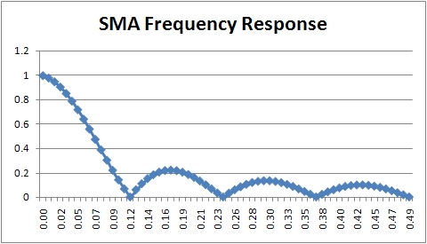
Where you can clearly see that the amount of signal transferred to the output after the cutoff frequency is very low.

Read More Articles on Time-series Forecasting